41. Another Look at the Kalman Filter #

GPU

This lecture is accelerated via hardware that has access to a GPU and JAX for GPU programming.

Free GPUs are available on Google Colab. To use this option, please click on the play icon top right, select Colab, and set the runtime environment to include a GPU.

Alternatively, if you have your own GPU, you can follow the instructions for installing JAX with GPU support. If you would like to install JAX running on the cpu only you can use pip install jax[cpu]

In this quantecon lecture A First Look at the Kalman filter, we used a Kalman filter to estimate locations of a rocket.

In this lecture, we’ll use the Kalman filter to infer a worker’s human capital and the effort that the worker devotes to accumulating human capital, neither of which the firm observes directly.

The firm learns about those things only by observing a history of the output that the worker generates for the firm, and from understanding how that output depends on the worker’s human capital and how human capital evolves as a function of the worker’s effort.

We’ll posit a rule that expresses how much the firm pays the worker each period as a function of the firm’s information each period.

In addition to what’s in Anaconda, this lecture will need the following libraries:

!pip install quantecon

To conduct simulations, we bring in these imports, as in A First Look at the Kalman filter.

import matplotlib.pyplot as plt
import numpy as np
import jax
import jax.numpy as jnp
from quantecon import Kalman, LinearStateSpace
from typing import NamedTuple
from scipy.stats import multivariate_normal
import matplotlib as mpl
mpl.rcParams['text.usetex'] = True
mpl.rcParams['text.latex.preamble'] = r'\usepackage{{amsmath}}'

Matplotlib is building the font cache; this may take a moment.

41.1. A worker’s output #

A representative worker is permanently employed at a firm.

The worker’s output is described by the following dynamic process:

(41.1)#\[\begin{split}\begin{aligned} h_{t+1} &= \alpha h_t + \beta u_t + c w_{t+1}, \quad w_{t+1} \sim {\mathcal N}(0,1) \\ u_{t+1} & = u_t \\ y_t & = g h_t + v_t , \quad v_t \sim {\mathcal N} (0, R) \end{aligned}\end{split}\]

Here

\(h_t\) is the logarithm of human capital at time \(t\)
\(u_t\) is the logarithm of the worker’s effort at accumulating human capital at \(t\)
\(y_t\) is the logarithm of the worker’s output at time \(t\)
\(h_0 \sim {\mathcal N}(\mu_{h, 0}, \sigma_{h,0})\)
\(u_0 \sim {\mathcal N}(\mu_{u, 0}, \sigma_{u,0})\)

Parameters of the model are \(\alpha, \beta, c, R, g, \mu_{h, 0}, \mu_{u, 0}, \sigma_{h,0}, \sigma_{u,0}\).

At time \(0\), a firm has hired the worker.

The worker is permanently attached to the firm and so works for the same firm at all dates \(t =0, 1, 2, \ldots\).

At the beginning of time \(0\), the firm observes neither the worker’s innate initial human capital \(h_0\) nor its hard-wired permanent effort level \(u_0\).

The firm believes that \(u_0\) for a particular worker is drawn from a Gaussian probability distribution, and so is described by \(u_0 \sim {\mathcal N}(\mu_{u, 0}, \sigma_{u,0})\).

The \(h_t\) part of a worker’s “type” moves over time, but the effort component of the worker’s type is \(u_t = u_0\).

This means that from the firm’s point of view, the worker’s effort is effectively an unknown fixed “parameter”.

At time \(t\geq 1\), for a particular worker the firm observed \(y^{t-1} = [y_{t-1}, y_{t-2}, \ldots, y_0]\).

The firm does not observe the worker’s “type” \((h_0, u_0)\).

But the firm does observe the worker’s output \(y_t\) at time \(t\) and remembers the worker’s past outputs \(y^{t-1}\).

41.2. A firm’s wage-setting policy #

Based on information about the worker that the firm has at time \(t \geq 1\), the firm pays the worker log wage

\[ w_t = g E [ h_t | y^{t-1} ], \quad t \geq 1 \]

and at time \(0\) pays the worker a log wage equal to the unconditional mean of \(y_0\):

\[ w_0 = g \mu_{h, 0} \]

In using this payment rule, the firm is taking into account that the worker’s log output today is partly due to the random component \(v_t\) that comes entirely from luck, and that is assumed to be independent of \(h_t\) and \(u_t\).

41.3. A state-space representation #

Write system (41.1) in the state-space form

\[\begin{aligned} \begin{bmatrix} h_{t+1} \cr u_{t+1} \end{bmatrix} &= \begin{bmatrix} \alpha & \beta \cr 0 & 1 \end{bmatrix} \begin{bmatrix} h_{t} \cr u_{t} \end{bmatrix} + \begin{bmatrix} c \cr 0 \end{bmatrix} w_{t+1} \cr y_t & = \begin{bmatrix} g & 0 \end{bmatrix} \begin{bmatrix} h_{t} \cr u_{t} \end{bmatrix} + v_t \end{aligned}\]

which is equivalent with

(41.2)#\[\begin{aligned} x_{t+1} & = A x_t + C w_{t+1} \cr y_t & = G x_t + v_t \cr x_0 & \sim {\mathcal N}(\mu_0, \Sigma_0) \end{aligned}\]

where

\[x_t = \begin{bmatrix} h_{t} \cr u_{t} \end{bmatrix} , \quad \mu_0 = \begin{bmatrix} \mu_{h ,0} \cr \mu_{u, 0} \end{bmatrix} , \quad \Sigma_0 = \begin{bmatrix} \sigma_{h,0} & 0 \cr 0 & \sigma_{u,0} \end{bmatrix}\]

To compute the firm’s wage-setting policy, we first create a NamedTuple to store the parameters of the model

class WorkerModel(NamedTuple):

    A: jax.Array
    C: jax.Array
    G: jax.Array
    R: jax.Array
    μ_0: jax.Array
    Σ_0: jax.Array


def create_worker(α=.8, β=.2, c=.2,
                  R=.5, g=1.0, μ_h=4, μ_u=4, 
                  σ_h=4, σ_u=4):
    
    A = jnp.array([[α, β], 
                   [0, 1]])
    C = jnp.array([[c], 
                   [0]])
    G = jnp.array([g, 0])
    R = jnp.array(R)

    # Define initial state and covariance matrix
    μ_0 = jnp.array([[μ_h], 
                     [μ_u]])
    
    Σ_0 = jnp.array([[σ_h, 0],
                     [0, σ_u]])
    
    return WorkerModel(A=A, C=C, G=G, R=R, μ_0=μ_0, Σ_0=Σ_0)

Please note how the WorkerModel namedtuple creates all of the objects required to compute an associated state-space representation (41.2).

This is handy, because in order to simulate a history \(\{y_t, h_t\}\) for a worker, we’ll want to form a state space system for him/her by using the LinearStateSpace class.

# Define A, C, G, R, μ_0, Σ_0
worker = create_worker()
A, C, G, R = worker.A, worker.C, worker.G, worker.R
μ_0, Σ_0 = worker.μ_0, worker.Σ_0

# Create a LinearStateSpace object
ss = LinearStateSpace(A, C, G, jnp.sqrt(R), 
                    mu_0=μ_0, Sigma_0=Σ_0)

T = 100
seed = 1234
x, y = ss.simulate(T, seed)
y = y.flatten()

h_0, u_0 = x[0, 0], x[1, 0]

Next, to compute the firm’s policy for setting the log wage based on the information it has about the worker, we use the Kalman filter described in this quantecon lecture A First Look at the Kalman filter.

In particular, we want to compute all of the objects in an “innovation representation”.

41.4. An Innovations representation #

We have all the objects in hand required to form an innovations representation for the output process \(\{y_t\}_{t=0}^T\) for a worker.

Let’s code that up now.

\[\begin{aligned} \hat x_{t+1} & = A \hat x_t + K_t a_t \cr y_{t} & = G \hat x_t + a_t \end{aligned}\]

where \(K_t\) is the Kalman gain matrix at time \(t\).

We accomplish this in the following code that uses the Kalman class.

x_hat_0, Σ_hat_0 = worker.μ_0, worker.Σ_0 # First guess of the firm
kalman = Kalman(ss, x_hat_0, Σ_hat_0)

x_hat = jnp.zeros((2, T))
Σ_hat = jnp.zeros((*Σ_0.shape, T))

# The data y[T] isn't used because we aren't making prediction about T+1
for t in range(1, T):
    kalman.update(y[t-1])
    x_hat_t, Σ_hat_t = kalman.x_hat, kalman.Sigma
    # x_hat_t = E(x_t | y^{t-1})
    x_hat = x_hat.at[:, t].set(x_hat_t.reshape(-1))
    Σ_hat = Σ_hat.at[:, :, t].set(Σ_hat_t)

# Add the initial
x_hat = x_hat.at[:, 0].set(x_hat_0.reshape(-1))
Σ_hat = Σ_hat.at[:, :, 0].set(Σ_hat_0)

# Compute other variables
y_hat = worker.G @ x_hat
u_hat = x_hat[1, :]

For a draw of \(h_0, u_0\), we plot \(E[y_t | y^{t-1}] = G \hat x_t \) where \(\hat x_t = E [x_t | y^{t-1}]\).

We also plot \(\hat u_t = E [u_t | y^{t-1}]\), which is the firm’s inference about a worker’s hard-wired “work ethic” \(u_0\), conditioned on information \(y^{t-1}\) that it has about him or her coming into period \(t\).

We can watch as the firm’s inference \(E [u_t | y^{t-1}]\) of the worker’s work ethic converges toward the hidden \(u_0\), which is not directly observed by the firm.

fig, ax = plt.subplots(1, 2)

ax[0].plot(y_hat, label=r'$E[y_t| y^{t-1}]$')
ax[0].set_xlabel('Time')
ax[0].set_ylabel(r'$E[y_t | y^{t-1}]$')
ax[0].set_title(r'$E[y_t | y^{t-1}]$ over time')
ax[0].legend()

ax[1].plot(u_hat, label=r'$E[u_t|y^{t-1}]$')
ax[1].axhline(y=u_0, color='grey', 
            linestyle='dashed', label=fr'$u_0={u_0:.2f}$')
ax[1].set_xlabel('Time')
ax[1].set_ylabel(r'$E[u_t|y^{t-1}]$')
ax[1].set_title('Inferred work ethic over time')
ax[1].legend()

fig.tight_layout()
plt.show()

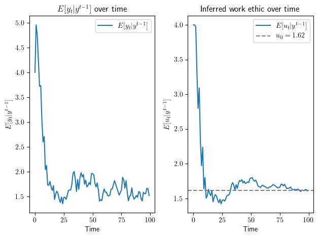
_images/ed9c1746f5e2bb40d3f6667737134039a544b291945fd709158a549568a4b85a.png — Fig. 41.1 Inferred variables using Kalman filter#

41.5. Some computational experiments #

Let’s look at \(\Sigma_0\) and \(\Sigma_T\) in order to see how much the firm learns about the hidden state during the horizon we have set.

print(Σ_hat[:, :, 0])

[[4. 0.]
 [0. 4.]]

print(Σ_hat[:, :, -1])

[[0.09403859 0.00997018]
 [0.00997018 0.01592704]]

Evidently, entries in the conditional covariance matrix become smaller over time.

It is enlightening to portray how conditional covariance matrices \(\Sigma_t\) evolve by plotting confidence ellipsoids around \(E [x_t |y^{t-1}] \) at various \(t\)’s.

# Create a grid of points for contour plotting
h_range = jnp.linspace(x_hat[0, :].min()-0.5*Σ_hat[0, 0, 1], 
                      x_hat[0, :].max()+0.5*Σ_hat[0, 0, 1], 100)
u_range = jnp.linspace(x_hat[1, :].min()-0.5*Σ_hat[1, 1, 1], 
                      x_hat[1, :].max()+0.5*Σ_hat[1, 1, 1], 100)
h, u = jnp.meshgrid(h_range, u_range)

# Create a figure with subplots for each time step
fig, axs = plt.subplots(1, 3, figsize=(12, 7))

# Iterate through each time step
for i, t in enumerate(np.linspace(0, T-1, 3, dtype=int)):
    # Create a multivariate normal distribution with x_hat and Σ at time step t
    mu = x_hat[:, t]
    cov = Σ_hat[:, :, t]
    mvn = multivariate_normal(mean=mu, cov=cov)
    
    # Evaluate the multivariate normal PDF on the grid
    pdf_values = mvn.pdf(np.dstack((h, u)))
    
    # Create a contour plot for the PDF
    con = axs[i].contour(h, u, pdf_values, cmap='viridis')
    axs[i].clabel(con, inline=1, fontsize=10)
    axs[i].set_title(f'Time Step {t+1}')
    axs[i].set_xlabel(r'$h_{{{}}}$'.format(str(t+1)))
    axs[i].set_ylabel(r'$u_{{{}}}$'.format(str(t+1)))
    
    cov_latex = (r'$\Sigma_{{{}}}= \begin{{bmatrix}} {:.2f} & {:.2f} \\ '
                 r'{:.2f} & {:.2f} \end{{bmatrix}}$'.format(
                     t+1, cov[0, 0], cov[0, 1], cov[1, 0], cov[1, 1]))
    axs[i].text(0.33, -0.15, cov_latex, transform=axs[i].transAxes)

    
plt.tight_layout()
plt.show()

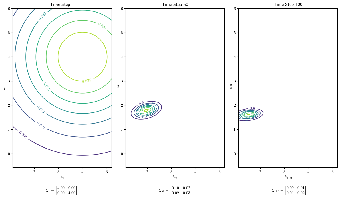
_images/131c3ed2827455f5eca6f3c4dbdf7ec9641cbe9006a7bfa2ee6deeef71ef1b26.png — Fig. 41.2 Confidence ellipsoid over updating#

Note how the accumulation of evidence \(y^t\) affects the shape of the confidence ellipsoid as sample size \(t\) grows.

Now let’s use our code to set the hidden state \(x_0\) to a particular vector in order to watch how a firm learns starting from some \(x_0\) we are interested in.

For example, let’s say \(h_0 = 0\) and \(u_0 = 4\).

Here is one way to do this.

# For example, we might want h_0 = 0 and u_0 = 4
ss_μ_0 = jnp.array([0.0, 4.0])

# Create a LinearStateSpace object with Sigma_0 as a matrix of zeros
ss_example = LinearStateSpace(A, C, G, np.sqrt(R), mu_0=ss_μ_0, 
                              # This line forces exact h_0=0 and u_0=4
                              Sigma_0=np.zeros((2, 2))
                             )

T = 100
seed = 1234
x, y = ss_example.simulate(T, seed)
y = y.flatten()

# Now h_0=0 and u_0=4
h_0, u_0 = x[0, 0], x[1, 0]
print('h_0 =', h_0)
print('u_0 =', u_0)

h_0 = 0.0
u_0 = 4.0

Another way to accomplish the same goal is to use the following code.

However, in this way we assume the underlying distribution of \(x_0\) has the mean \(\mu_0 = (0, 4)\top\).

# If we want to set the initial 
# h_0 = μ_h = 0 and u_0 = μ_u = 4.0:
worker = create_worker(μ_h=0.0, μ_u=4.0)

ss_example = LinearStateSpace(A, C, G, np.sqrt(R), 
                              # This line takes h_0=μ_h and u_0=μ_u
                              mu_0=worker.μ_0,
                              # This line forces exact h_0=μ_h and u_0=μ_u
                              Sigma_0=np.zeros((2, 2))
                             )

T = 100
seed = 1234
x, y = ss_example.simulate(T, seed)
y = y.flatten()

# Now h_0 and u_0 will be exactly μ_0
h_0, u_0 = x[0, 0], x[1, 0]
print('h_0 =', h_0)
print('u_0 =', u_0)

h_0 = 0.0
u_0 = 4.0

For this worker, let’s generate a plot like the one above.

# First we compute the Kalman filter with initial x_hat_0 and Σ_hat_0 
x_hat_0, Σ_hat_0 = worker.μ_0, worker.Σ_0
kalman = Kalman(ss, x_hat_0, Σ_hat_0)

x_hat = jnp.zeros((2, T))
Σ_hat = jnp.zeros((*Σ_0.shape, T))

# Then we iteratively update the Kalman filter class using 
# observation y based on the linear state model above:
for t in range(1, T):
    kalman.update(y[t-1])
    x_hat_t, Σ_hat_t = kalman.x_hat, kalman.Sigma

    x_hat = x_hat.at[:, t].set(x_hat_t.reshape(-1))
    Σ_hat = Σ_hat.at[:, :, t].set(Σ_hat_t)

# Add the initial
x_hat = x_hat.at[:, 0].set(x_hat_0.reshape(-1))
Σ_hat = Σ_hat.at[:, :, 0].set(Σ_hat_0)

# Compute other variables
y_hat = worker.G @ x_hat
u_hat = x_hat[1, :]

# Generate plots for y_hat and u_hat
fig, ax = plt.subplots(1, 2)

ax[0].plot(y_hat, label=r'$E[y_t| y^{t-1}]$')
ax[0].set_xlabel('Time')
ax[0].set_ylabel(r'$E[y_t | y^{t-1}]$')
ax[0].set_title(r'$E[y_t | y^{t-1}]$ over time')
ax[0].legend()

ax[1].plot(u_hat, label=r'$E[u_t|y^{t-1}]$')
ax[1].axhline(y=u_0, color='grey', 
            linestyle='dashed', label=fr'$u_0={u_0:.2f}$')
ax[1].set_xlabel('Time')
ax[1].set_ylabel(r'$E[u_t|y^{t-1}]$')
ax[1].set_title('Inferred work ethic over time')
ax[1].legend()

fig.tight_layout()
plt.show()

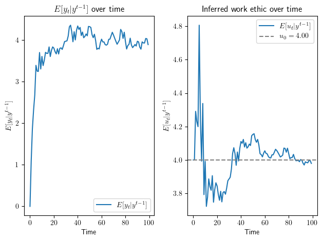
_images/222fc023a7e48805d47123a2fae5cc1234804f7cd09b4acd2d12bc30051f42c4.png — Fig. 41.3 Inferred variables with fixing initial#

More generally, we can change some or all of the parameters defining a worker in our create_worker namedtuple.

Here is an example.

# We can set these parameters when creating a worker -- just like classes!
hard_working_worker = create_worker(α=.4, β=.8, 
                        μ_h=7.0, μ_u=100, σ_h=2.5, σ_u=3.2)

print(hard_working_worker)

WorkerModel(A=Array([[0.4, 0.8],
       [0. , 1. ]], dtype=float32), C=Array([[0.2],
       [0. ]], dtype=float32), G=Array([1., 0.], dtype=float32), R=Array(0.5, dtype=float32, weak_type=True), μ_0=Array([[  7.],
       [100.]], dtype=float32), Σ_0=Array([[2.5, 0. ],
       [0. , 3.2]], dtype=float32))

We can also simulate the system for \(T = 50\) periods for different workers.

The difference between the inferred work ethics and true work ethics converges to \(0\) over time.

This shows that the filter is gradually teaching the worker and firm about the worker’s effort.

num_workers = 3
T = 50
fig, ax = plt.subplots(figsize=(7, 7))

for i in range(num_workers):
    worker = create_worker(μ_u=4+2*i)
    simulate_workers(worker, T, ax, seed=1234+i)
ax.set_ylim(ymin=-2, ymax=2)
plt.show()

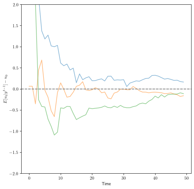
_images/adf26d6f69da36fd24a5a04ef45445e33e482c11c3a7da70ca998dc19d97f2a4.png — Fig. 41.4 Difference between inferred and true ethic#

# We can also generate plots of u_t:

T = 50
fig, ax = plt.subplots(figsize=(7, 7))

μ_us = [2, -2, 1]
αs = [0.2, 0.3, 0.5]
βs = [0.1, 0.9, 0.3]

for i, (μ_u, α, β) in enumerate(zip(μ_us, αs, βs)):
    worker = create_worker(μ_u=μ_u, α=α, β=β)
    simulate_workers(worker, T, ax,
                    # By setting diff=False, it will give u_t
                    diff=False, name=r'$u_{{{}, t}}$'.format(i),
                    seed=1234+i)

ax.legend(bbox_to_anchor=(1, 0.5))
plt.show()

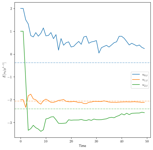
_images/c3922e8e7e2fbfcbfbf61ee7ba4f90d1d801543bffc78aa42f469333536410bc.png — Fig. 41.5 Inferred work ethic over time#

# We can also use exact u_0=1 and h_0=2 for all workers

T = 50
fig, ax = plt.subplots(figsize=(7, 7))

# These two lines set the generated u_0=1 and h_0=2 for all workers
ss_μ = jnp.array([[1],
                  [2]])
ss_Σ = jnp.zeros((2,2))

μ_us = [2, -2, 1]
αs = [0.2, 0.3, 0.5]
βs = [0.1, 0.9, 0.3]

for i, (μ_u, α, β) in enumerate(zip(μ_us, αs, βs)):
    worker = create_worker(μ_u=μ_u, α=α, β=β)
    simulate_workers(worker, T, ax, ss_μ=ss_μ, ss_Σ=ss_Σ, 
                     diff=False, name=r'$u_{{{}, t}}$'.format(i),
                     seed=1234+i)
    
# This controls the boundary of plots
ax.set_ylim(ymin=-3, ymax=3)
ax.legend(bbox_to_anchor=(1, 0.5))
plt.show()

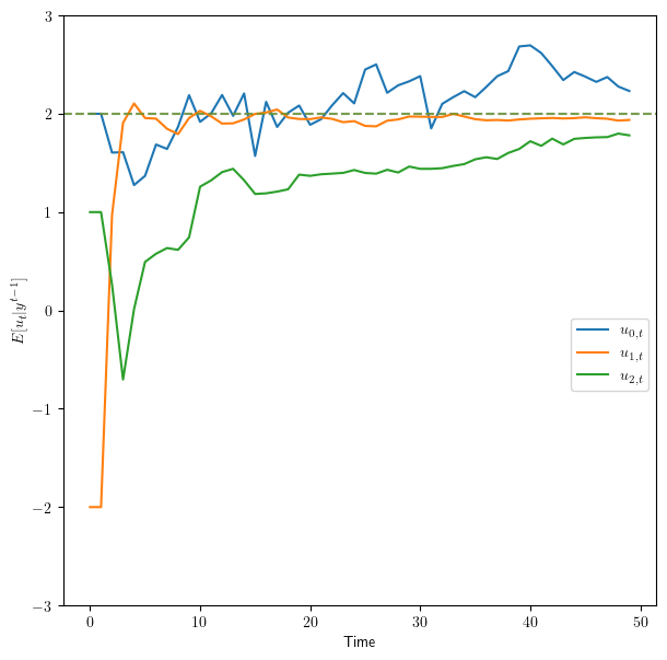
_images/edab6dd8ffde930ef7ec6dbf89c0b89ccc6a6ef93a1e4247ffabf97c7e92879e.png — Fig. 41.6 Inferred ethic with fixed initial#

# We can generate a plot for only one of the workers:

T = 50
fig, ax = plt.subplots(figsize=(7, 7))

ss_μ_1 = np.array([[1],
                   [100]])
ss_μ_2 = np.array([[1],
                   [30]])
ss_Σ = np.zeros((2,2))

μ_us = 100
αs = 0.5
βs = 0.3

worker = create_worker(μ_u=μ_us, α=α, β=β)
simulate_workers(worker, T, ax, ss_μ=ss_μ_1, ss_Σ=ss_Σ, 
                 diff=False, name=r'Hard-working worker')
simulate_workers(worker, T, ax, ss_μ=ss_μ_2, ss_Σ=ss_Σ, 
                 diff=False, 
                 title='A hard-working worker and a less hard-working worker',
                 name=r'Normal worker')
ax.axhline(y=u_0, xmin=0, xmax=0, color='grey', 
           linestyle='dashed', label=r'$u_{i, 0}$')
ax.legend(bbox_to_anchor=(1, 0.5))
plt.show()

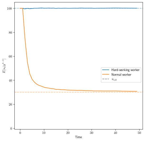
_images/175c7af69a68470d7a29229ed0c88851ff41f710b1abfd261f07087bc23ff54b.png — Fig. 41.7 Inferred ethic with two fixed initial#

41.6. Future extensions #

We can do lots of enlightening experiments by creating new types of workers and letting the firm learn about their hidden (to the firm) states by observing just their output histories.

41. Another Look at the Kalman Filter#

41.1. A worker’s output#

41.2. A firm’s wage-setting policy#

41.3. A state-space representation#

41.4. An Innovations representation#

41.5. Some computational experiments#

41.6. Future extensions#